NACA0012 Tutorial

This tutorial is a walkthrough for the panel method. We will be using the ex_1_NACA0012.py example.

We begin by importing relevant packages. We use numpy as the standard library for general arrays. We also import csdl to set up the graph.

Next, we import the PanelMethod flow solver class from VortexAD. We also use one of the stored meshes, which can be accessed through the SAMPLE_GEOMETRY_PATH path. We use this path to access the mesh for this tutorial.

import numpy as np
import csdl_alpha as csdl

from VortexAD import PanelMethod
from VortexAD import SAMPLE_GEOMETRY_PATH

Next, we instantiate the graph recorder and set up inputs to the flow solver. The Recorder object is used to start the graph assembly. The inline argument dictates whether values will be stored with the graph assembly (True) or if only the graph structure will be formed (False).

From there, we set up our panel method inputs. First, we need to supply a path to the mesh file. We use the NACA0012 stl mesh made using OpenVSP, with clustering at the leading and trailing edges. In addition, we set up a variable for the pitch angle in degrees. We do this to easily control

Next, we add the inputs we want to control into a dictionary to be read by the flow solver. In this case, we control two flow properties: the Mach number and pitch angle. We supply the mesh path, along with a reference area for our force and moment coefficients.

# instantiate recorder to assemble the graph
recorder = csdl.Recorder(inline=False)
recorder.start()

# set up input dictionary
mesh_file_path = str(SAMPLE_GEOMETRY_PATH) + '/pm/naca0012_LE_TE_cluster.stl'
pitch = csdl.Variable(value=np.array([5.]))

# input dict
input_dict = {
    'Mach': 0.25,
    'alpha': pitch,
    'Cp cutoff': -5.,
    'mesh_path': mesh_file_path, # can alternatively load mesh in with connectivity/TE data
    'ref_area': 10., 
}

Once our inputs are set up, we instantiate the flow solver and declare outputs.

We use the .declare_outputs() method to specify which outputs of the panel method we are interested in. The available outputs can be found at the link here or by calling .print_output_options(). For this tutorial, we are interested in the lift and induced drag coefficients, along with the pressure coefficient distribution.

In addition, we manually call the .setup_grid_properties() method to verify the grid and trailing edge selection. Although this method is automatically called during instantiation of thePanelMethod class, we call it manually here to highlight this capability. Potential flow methods require specifying trailing edge locations (where wakes will shed from), so it is important to mark these elements accurately. The threshold_angle argument specifies the sharpness angle between adjacent panels, and the plot argument can be used to visualize the grid.

Once our outputs have been set up, we can run through the panel method and assemble the graph by calling the .evaluate() method, which returns a dictionary of the outputs we previously declared. From there, we can extract our outputs of interested based on name.

Warning

Because we have set inline=False in the recorder, printing out these variables (CL, CDi, CP) will return nothing. We will need to use one of the backends to execute the graph to return its value.

# instantiate PanelMethod class
panel_method = PanelMethod(
    input_dict
)
# declare outputs of interest
pm_outputs = [
    'CL',
    'CDi',
    'Cp'
]
panel_method.declare_outputs(pm_outputs)

panel_method.setup_grid_properties(threshold_angle=125, plot=True) # optional for debugging

# run the panel method
outputs = panel_method.evaluate()

# read outputs
CL = outputs['CL']
CDi = outputs['CDi']
CP = outputs['Cp']

(810, 3)
(1, 810, 3)
running pre-processing
solving for doublet strengths
yes batching; batch size = 1
running post-processor
(1,)

/home/luca/Packages/csdl_alpha/csdl_alpha/src/operations/tensor/expand.py:184: UserWarning: "action" will have no effect when expanding a scalar.
  warnings.warn('"action" will have no effect when expanding a scalar.')

the panel method will print some statements during graph assembly, such as different stages of the internal graph structure. In this case, we are also using partitioned vectorization, so the partition size is printed.

Once the panel method graph has been assembled and CSDL variables have been assigned to python variables, we instantiate up a backend to compile and execute the graph. We use the JaxSimulator, which compiles the CSDL graph into jax code. We first need to set up lists for the graph inputs and outputs. These inputs and outputs are important because they identify what we have access to once the graph is compiled. To be more specific, once the graph is compiled, we can only change the variables in the input list to see only the variables in the output list. From there, we can execute the graph by calling sim.run().

# csdl-jax stuff
inputs = [pitch]
outputs = [CL, CDi, CP]

sim = csdl.experimental.JaxSimulator(
    recorder=recorder,
    additional_inputs=inputs,
    additional_outputs=outputs,
    gpu=False
)
sim.run()

compiling 'run' function ... (2168 nodes)

{<csdl_alpha.src.graph.variable.Variable at 0x70fff8194c70>: array([0.44523591]),
 <csdl_alpha.src.graph.variable.Variable at 0x70fff8194ee0>: array([0.00544886]),
 <csdl_alpha.src.graph.variable.Variable at 0x70fff81319d0>: array([[ 0.27168939,  0.2194987 ,  0.19842159, ..., -5.        ,
         -5.        , -5.        ]])}

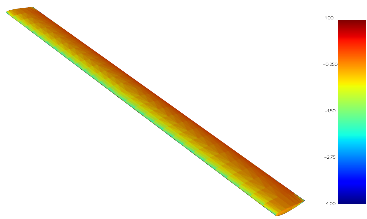
Once the simulator runs, we can see the values of our three outputs. In addition, we use the plotting functionality in the PanelMethod class to plot our pressure distribution over the geometry.

CL_val = sim[CL]
CDi_val = sim[CDi]
CP_val = sim[CP]

print('CL:', CL_val)
print('CDi:', CDi_val)

panel_method.plot(CP_val, bounds=[-4,1])

CL: [0.44523591]
CDi: [0.00544886]